In this story we will learn how to write a simple gaussian fit to a dataset using the least square method.
Let us say we have a dataset plotted resembling the one below for which we have singled out a normal distribution:
Normal distribution
We know the equation of the curve:
Eq. 1
We have:
Eq. 2
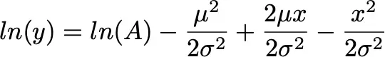
I will let you do the math and rewrite this as:
Eq. 3
Now if I have a dataset, I will be able to assess the error between Eq. 3 and the dataset by doing this operation:
Eq. 4
I can even sum the errors for each point or datum. What if the negatives cancel the positives? I do not want that, so it would better to sum the squares of the errors ∑ δ² .
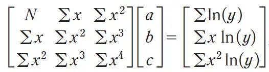
Now to plot my gaussian, I would want the values a, b, c. I would then need to minimize ∑ δ² with respect to the variables a, b, c (I would be minimizing the error by setting the derivatives of ∑ δ² with respect to a, b, c, to zero). Doing so would result in obtaining a set of equations that one would put in the form of a matrix (N is the number of points). Do the math :):
Eq. 5
How would we fit with python? We need to solve the matrix expression
Mx = P. We assume we have an excel file to analyze, we open the file:
import pandas as pd import numpy as np from pandas import ExcelWriter from pandas import ExcelFile
Assume we have df[0] for x and df[1] for y. We create each entry of the matrix:
a1 = len(df) # N
a2 = (df[0]).sum() # sum of x
a3 = (df[0]**2).sum() # sum of x^2
A = np.log(df[1]).sum() # sum of ln(y)
a4 = (df[0]).sum() # sum of x
a5 = (df[0]**2).sum() # sum of x^2
a6 = (df[0]**3).sum() # sum of x^3
B = ((df[0])*np.log(df[1])).sum() # sum x ln(y)
a7 = (df[0]**2).sum() # sum of x^2
a8 = (df[0]**3).sum() # sum of x^3
a9 = (df[0]**4).sum() # sum of x^4
C =((df[0]**2)*np.log(df[1])).sum() # sum x^2 ln(y)
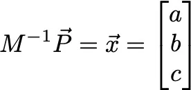
We set our matrix and solve either with the LU method or inverse matrix method whichever is best for you:
Eq. 6
import scipy.linalg as linalg

M = np.array([[a1, a2, a3], [a4, a5, a6], [a7, a8, a9]]) # the matrix M
P = np.array([A, B, C]) # the vector P

LU = linalg.lu_factor(M)
x2 = linalg.lu_solve(LU, P) # x2 is the vector [a, b, c]
x1 = np.linalg.solve(M, P) # x1 is the vector [a, b, c]
We can later on convert the values a, b, c to their equivalent in Eq. 2.
This a simple fitting that does not do great with noise, long tail etc. However it will do the job. There is multiple ways to reduce the error based on these math principles (the Caruana’s algorithm).
This it! Try it yourself! Get your data, plot them, fit them and compare the plots!